Blog¶

June 10, 2024
in SageMaker, AI
8 min read

Draft

SageMaker Deployment Options

Basics

Sagemaker Domain

Amazon SageMaker uses domains to organize user profiles, applications, and their associated resources. An Amazon SageMaker domain consists of the following:

An associated Amazon Elastic File System (Amazon EFS) volume.
A list of authorized users.
A variety of security, application, policy, and Amazon Virtual Private Cloud (Amazon VPC) configurations.

Studio vs Notebook Instance 🗒️

Notebooks are jupyter notebook where resource allocation are done by AWS. So they are fully managed
Studio is IDE which is not fully managed

Features

Prepare 🧑‍🍳

Ground Truth: Enable DS to label jobs, datasets and workforces.
Clarify: Detect bias and understand model predictions.
Data wrangler: Filtering, joining and other data preparation tasks.

Build 👷

Autopilot: Automatically create models
Built-in:
JumpStart:

Train 🚊

Experiments:
Managed Train: Fully managed training by AWS to reduce the cost.
Distributed training:

Deploy 🚟

Model Monitoring:
Endpoints: Multi model endpoint, Multi container endpoint.
Inference: Based on traffic patterns, we can have following
Real time: For persistent, one prediction at time
Serverless: Workloads which can tolerate idle periods between spikes and can tolerate cold starts
Batch: To get predictions for an entire dataset, use SageMaker batch transform
Async: Requests with large payload sizes up to 1GB, long processing times, and near real-time latency requirements, use Amazon SageMaker Asynchronous Inference

Batch inference refers to model inference performed on data that is in batches, often large batches, and asynchronous in nature. It fits use cases that collect data infrequently, that focus on group statistics rather than individual inference, and that do not need to have inference results right away for downstream processes.

Projects that are research oriented, for example, do not require model inference to be returned for a data point right away. Researchers often collect a chunk of data for testing and evaluation purposes and care about overall statistics and performance rather than individual predictions. They can conduct the inference in batches and wait for the prediction for the whole batch to complete before they move on

Doing batch transform in S3 🪣

Depending on how you organize the data, SageMaker batch transform can split a single large text file in S3 by lines into a small and manageable size (mini-batch) that would fit into the memory before making inference against the model; it can also distribute the files by S3 key into compute instances for efficient computation.

SageMaker batch transform saves the results after assembly to the specified S3 location with .out appended to the input filename.

Async Transformation ⚙️

Amazon SageMaker Asynchronous Inference is a capability in SageMaker that queues incoming requests and processes them asynchronously. This option is ideal for requests with large payload sizes (up to 1GB), long processing times (up to one hour), and near real-time latency requirements. Asynchronous Inference enables you to save on costs by autoscaling the instance count to zero when there are no requests to process, so you only pay when your endpoint is processing requests.

Real-time Inference ⏳

In today's fast-paced digital environment, receiving inference results for incoming data points in real-time is crucial for effective decision-making.

Take interactive chatbots, for instance; they rely on live inference capabilities to operate effectively. Users expect instant responses during their conversations—waiting until the discussion is over or enduring delays of even a few seconds is simply not acceptable.

For companies striving to deliver top-notch customer experiences, ensuring that inferences are generated and communicated to customers instantly is a top priority.

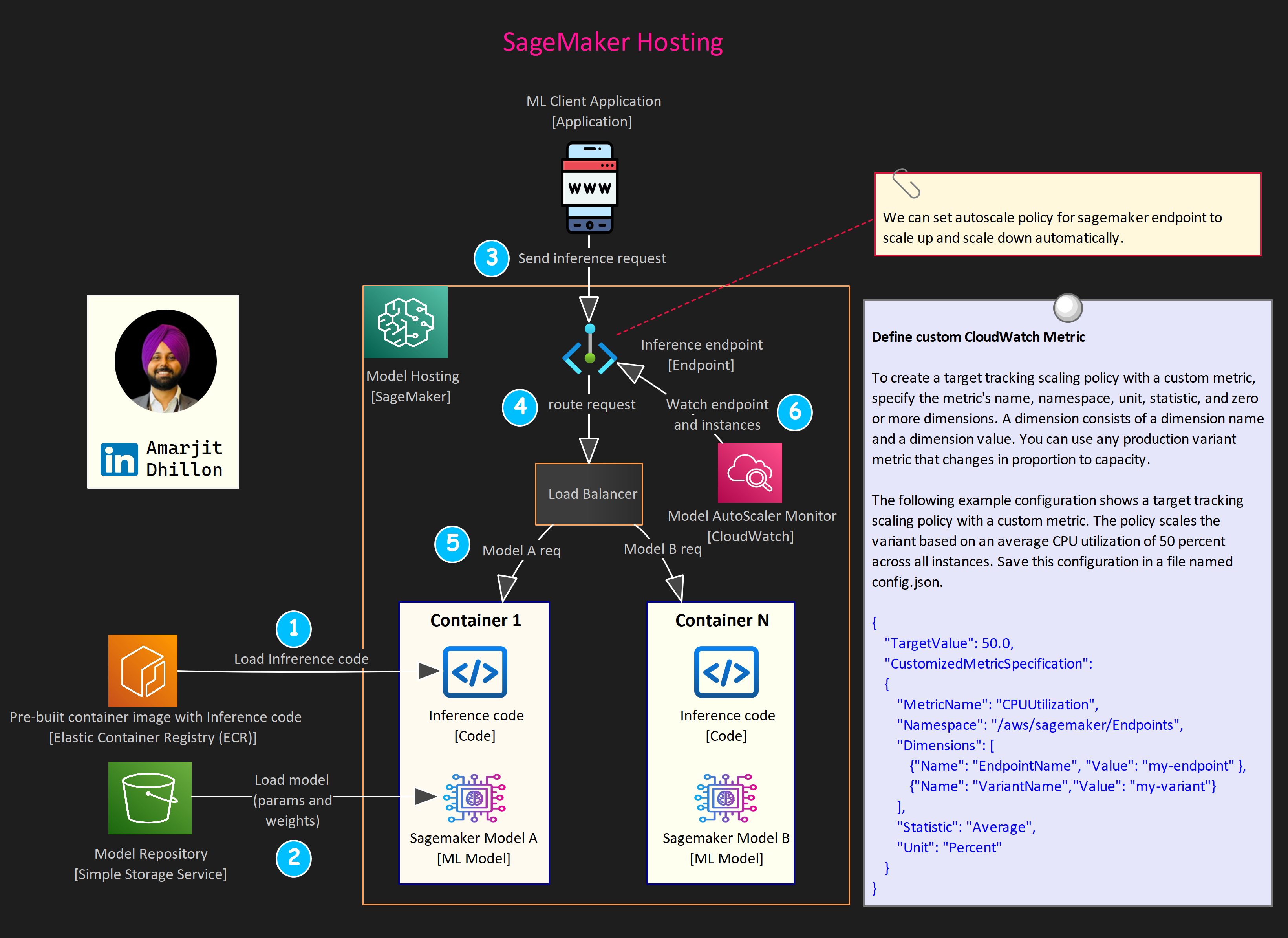
Host real-time endpoints

The deployment process consists of the following steps:

Create a model, container, and associated inference code in SageMaker. The model refers to the training artifact, model.tar.gz. The container is the runtime environment for the code and the model.
Create an HTTPS endpoint configuration. This configuration carries information about compute instance type and quantity, models, and traffic patterns to model variants.
Create ML instances and an HTTPS endpoint. SageMaker creates a fleet of ML instances and an HTTPS endpoint that handles the traffic and authentication. The final step is to put everything together for a working HTTPS endpoint that can interact with client-side requests.

Serverless Inference 🖥️

On-demand Serverless Inference is ideal for workloads which have idle periods between traffic spurts and can tolerate cold starts. Serverless endpoints automatically launch compute resources and scale them in and out depending on traffic, eliminating the need to choose instance types or manage scaling policies. This takes away the undifferentiated heavy lifting of selecting and managing servers.

Serverless Inference integrates with AWS Lambda to offer you high availability, built-in fault tolerance and automatic scaling. With a pay-per-use model, Serverless Inference is a cost-effective option if you have an infrequent or unpredictable traffic pattern.

During times when there are no requests, Serverless Inference scales your endpoint down to 0, helping you to minimize your costs.

Invoke Serverless Endpoint

runtime = boto3.client("sagemaker-runtime")

endpoint_name = "<your-endpoint-name>"
content_type = "<request-mime-type>"
payload = <your-request-body>

response = runtime.invoke_endpoint(
    EndpointName=endpoint_name,
    ContentType=content_type,
    Body=payload
)

Possible cold-start during updating serverless endpoint

Note that when updating your endpoint, you can experience cold starts when making requests to the endpoint because SageMaker must re-initialize your container and model.

response = client.update_endpoint(
  EndpointName="<your-endpoint-name>",
  EndpointConfigName="<new-endpoint-config>",
)

Use Provisioned Concurrency

Amazon SageMaker automatically scales in or out on-demand serverless endpoints. For serverless endpoints with Provisioned Concurrency you can use Application Auto Scaling to scale up or down the Provisioned Concurrency based on your traffic profile, thus optimizing costs.

Optimizations

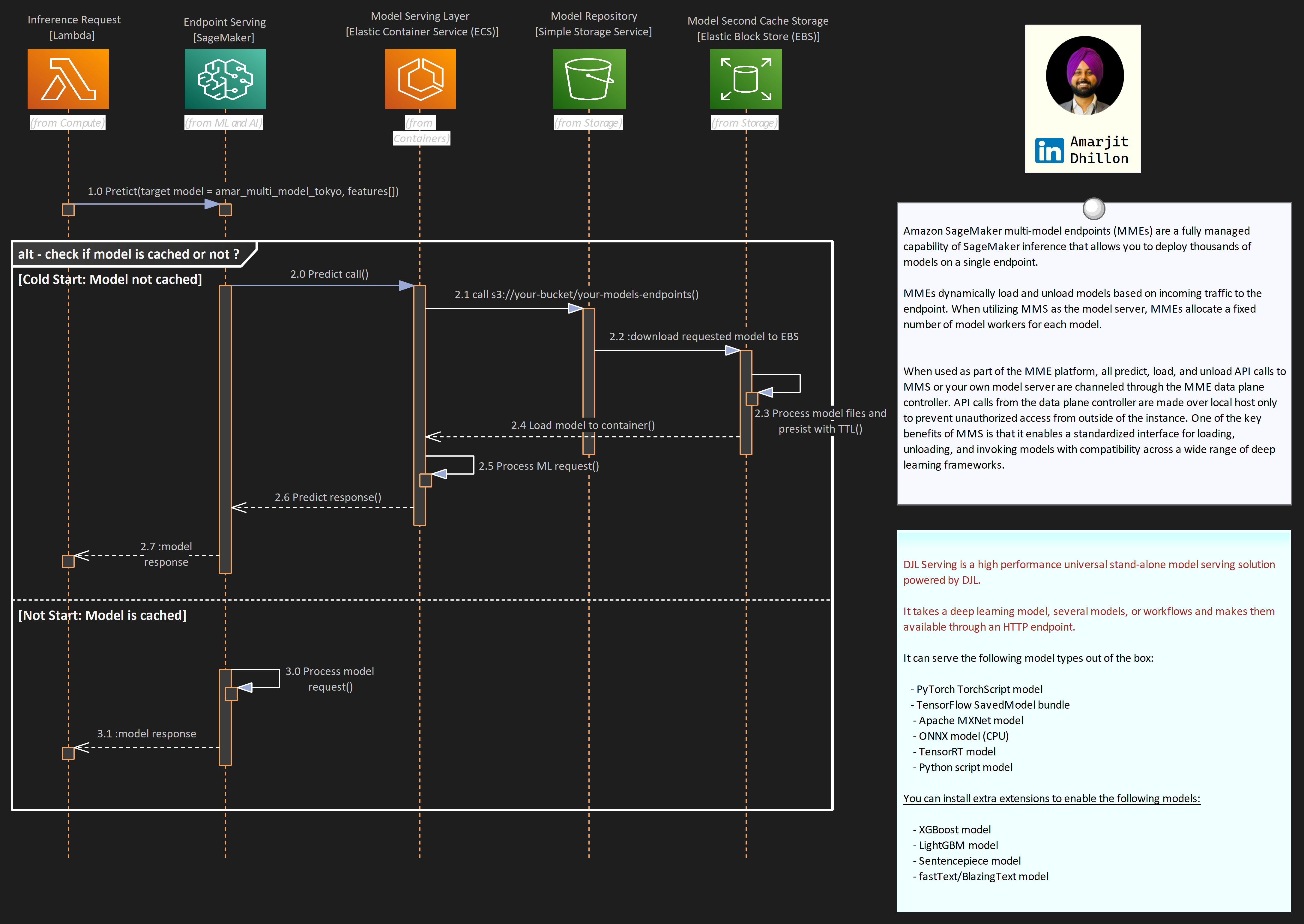
Multi Model Endpoints ⟜

Amazon SageMaker multi-model endpoint (MME) enables you to cost-effectively deploy and host multiple models in a single endpoint and then horizontally scale the endpoint to achieve scale.

When to use MME?

Multi-model endpoints are suitable for use cases where you have models that are built in the same framework (XGBoost in this example), and where it is tolerable to have latency on less frequently used models.

As illustrated in the following figure, this is an effective technique to implement multi-tenancy of models within your machine learning (ML) infrastructure.

Use Cases

Shared tenancy: SageMaker multi-model endpoints are well suited for hosting a large number of models that you can serve through a shared serving container and you don’t need to access all the models at the same time. Depending on the size of the endpoint instance memory, a model may occasionally be unloaded from memory in favor of loading a new model to maximize efficient use of memory, therefore your application needs to be tolerant of occasional latency spikes on unloaded models.

Co host models: MME is also designed for co-hosting models that use the same ML framework because they use the shared container to load multiple models. Therefore, if you have a mix of ML frameworks in your model fleet (such as PyTorch and TensorFlow), SageMaker dedicated endpoints or multi-container hosting is a better choice.

Ability to handle cold starts: Finally, MME is suited for applications that can tolerate an occasional cold start latency penalty, because models are loaded on first invocation and infrequently used models can be offloaded from memory in favor of loading new models. Therefore, if you have a mix of frequently and infrequently accessed models, a multi-model endpoint can efficiently serve this traffic with fewer resources and higher cost savings.

Host both CPU and GPU: Multi-model endpoints support hosting both CPU and GPU backed models. By using GPU backed models, you can lower your model deployment costs through increased usage of the endpoint and its underlying accelerated compute instances.

Advanced Configs

Increase inference parallelism per model

MMS creates one or more Python worker processes per model based on the value of the default_workers_per_model configuration parameter. These Python workers handle each individual inference request by running any preprocessing, prediction, and post processing functions you provide.

Design for spikes

Each MMS process within an endpoint instance has a request queue that can be configured with the job_queue_size parameter (default is 100). This determines the number of requests MMS will queue when all worker processes are busy. Use this parameter to fine-tune the responsiveness of your endpoint instances after you’ve decided on the optimal number of workers per model.

Setup AutoScaling

Before you can use auto scaling, you must have already created an Amazon SageMaker model endpoint. You can have multiple model versions for the same endpoit. Each model is referred to as a production (model) variant.

Setup cooldown policy

A cooldown period is used to protect against over-scaling when your model is scaling in (reducing capacity) or scaling out (increasing capacity). It does this by slowing down subsequent scaling activities until the period expires. Specifically, it blocks the deletion of instances for scale-in requests, and limits the creation of instances for scale-out requests.

Muti-container Endpoints ⋺

SageMaker multi-container endpoints enable customers to deploy multiple containers, that use different models or frameworks (XGBoost, Pytorch, TensorFlow), on a single SageMaker endpoint.

The containers can be run in a sequence as an inference pipeline, or each container can be accessed individually by using direct invocation to improve endpoint utilization and optimize costs.

Load Testing 🚛

Load testing is a technique that allows us to understand how our ML model hosted in an endpoint with a compute resource configuration responds to online traffic.

There are factors such as model size, ML framework, number of CPUs, amount of RAM, autoscaling policy, and traffic size that affect how your ML model performs in the cloud. Understandably, it's not easy to predict how many requests can come to an endpoint over time.

It is prudent to understand how your model and endpoint behave in this complex situation. Load testing creates artificial traffic and requests to your endpoint and stress tests how your model and endpoint respond in terms of model latency, instance CPU utilization, memory footprint, and so on.

Elastic Interface (EI)

EI attaches fractional GPUs to a SageMaker hosted endpoint. It increases the inference throughput and decreases the model latency for your deep learning models that can benefit from GPU acceleration

SageMaker Neo 👾

Neo is a capability of Amazon SageMaker that enables machine learning models to train once and run anywhere in the cloud and at the edge.

Why use NEO

Problem Statement

Generally, optimizing machine learning models for inference on multiple platforms is difficult because you need to hand-tune models for the specific hardware and software configuration of each platform. If you want to get optimal performance for a given workload, you need to know the hardware architecture, instruction set, memory access patterns, and input data shapes, among other factors. For traditional software development, tools such as compilers and profilers simplify the process. For machine learning, most tools are specific to the framework or to the hardware. This forces you into a manual trial-and-error process that is unreliable and unproductive.

Solution

Neo automatically optimizes Gluon, Keras, MXNet, PyTorch, TensorFlow, TensorFlow-Lite, and ONNX models for inference on Android, Linux, and Windows machines based on processors from Ambarella, ARM, Intel, Nvidia, NXP, Qualcomm, Texas Instruments, and Xilinx. Neo is tested with computer vision models available in the model zoos across the frameworks. SageMaker Neo supports compilation and deployment for two main platforms:

Cloud instances (including Inferentia)
Edge devices.

EC2 inf1 instances 🍪

Inf1 provide high performance and low cost in thecloud with AWS Inferentia chips designed and built by AWS for ML inference purposes.You can compile supported ML models using SageMaker Neo and select Inf1 instances todeploy the compiled model in a SageMaker hosted endpoint.

Optimize LLM's on Sagemaker

LMI containers 🚢

LMI containers are a set of high-performance Docker Containers purpose built for large language model (LLM) inference.

With these containers, you can leverage high performance open-source inference libraries like vLLM, TensorRT-LLM, Transformers NeuronX to deploy LLMs on AWS SageMaker Endpoints. These containers bundle together a model server with open-source inference libraries to deliver an all-in-one LLM serving solution.

June 10, 2024
in RAG, GenAI, Vector DB, Embeddings, LLM
2 min read

Draft

Vector Databases ➾

A vector database is specifically designed to operate on embedding vectors. As the popularity of LLMs and generative AI has grown recently, so has the use of embeddings to encode unstructured data. Vector databases have emerged as an effective solution for enterprises to deliver and scale these use cases.

What is Vector DB?

Vector databases are specialized databases that store data as high-dimensional vectors and their original content. They offer the capabilities of both vector indexes and traditional databases, such as optimized storage, scalability, flexibility, and query language support. They allow users to find and retrieve similar or relevant data based on their semantic or contextual meaning.

Vector databases can help RAG models quickly find the most similar documents or passages to a given query and use them as additional context for the LLM.

Vector Index

A vector index is a data structure in a vector database designed to enhance the efficiency of processing, and it is particularly suited for the high-dimensional vector dataencountered with LLMs. Its function is to streamline the search and retrieval processes within the database.

By implementing a vector index, the system is capable ofconducting quick similarity searches, identifying vectors that closely match or aremost similar to a given input vector.

How to convert embedding to vector index?

To create vector indexes for your embeddings, there are many options, such as exact or approximate nearest neighbor algorithms (e.g., HNSW or IVF), different distance metrics (e.g., cosine or Euclidean), or various compression techniques (e.g.,quantization or pruning).

Vector Search

A vector search is used to find the most relevant documents or passages to the query based on the similarity between the query vector and the document vectors in the index.

Similarity measures are mathematical methods that compare two vectors and compute a distance value between them. This distance value indicates how dissimilar or similar the two vectors are in terms of their semantic meaning

June 7, 2023
in Architecture, Databricks
5 min read

Draft

Manipulating Tables with Delta Lake 🐟

In this blog post, we’re going to explore how to effectively manage and manipulate tables using Delta Lake. Whether you're new to Delta Lake or need a refresher, this hands-on guide will take you through the essential operations needed to work with Delta tables.

From creating tables to updating and deleting records, we’ve got you covered! So, let’s dive in and get started! 🚀

Learning Objectives 🧩

By the end of this lab, you should be able to execute standard operations to create and manipulate Delta Lake tables, including:

Creating tables
Inserting data
Selecting records
Updating values
Deleting rows
Merging data
Dropping tables

Setup ⚙️

Before we jump into the fun part, let’s clear out any previous runs of this notebook and set up the necessary environment. Run the script below to reset and prepare everything.

%run ../Includes/Classroom-Setup-2.2L

Create Table ➕

We'll kick things off by creating a Delta Lake table that will track our favorite beans collection. The table will include a few basic fields to describe each bean.

Field Name	Field type
name	STRING
color	STRING
grams	FLOAT
delicious	BOOLEAN

Let’s go ahead and create the beans table with the following schema:

create table beans 
(name string, color string, grams float, delicious boolean)

Note

We'll use Python to run checks occasionally throughout the lab. The following cell will return as error with a message on what needs to change if you have not followed instructions. No output from cell execution means that you have completed this step.

assert spark.table("beans"), "Table named `beans` does not exist"
assert spark.table("beans").columns == ["name", "color", "grams", "delicious"], "Please name the columns in the order provided above"
assert spark.table("beans").dtypes == [("name", "string"), ("color", "string"), ("grams", "float"), ("delicious", "boolean")], "Please make sure the column types are identical to those provided above"

Insert Data 📇

Next, let’s populate the table with some data. The following SQL command will insert three records into our table.

INSERT INTO beans VALUES
("black", "black", 500, true),
("lentils", "brown", 1000, true),
("jelly", "rainbow", 42.5, false)

To make sure that the data was inserted correctly, let’s query the table to review the contents:

select * from beans

Now, let’s add a few more records in one transaction:

insert into beans values
('pinto', 'brown', 1.5, true),
('green', 'green', 178.3, true),
('beanbag chair', 'white', 40000, false)

Verify the data is in the correct state using the cell below:

assert spark.conf.get("spark.databricks.delta.lastCommitVersionInSession") == "2", "Only 3 commits should have been made to the table"
assert spark.table("beans").count() == 6, "The table should have 6 records"
assert set(row["name"] for row in spark.table("beans").select("name").collect()) == {'beanbag chair', 'black', 'green', 'jelly', 'lentils', 'pinto'}, "Make sure you have not modified the data provided"

Update Records 📢

Now, let's update some of our data. A friend pointed out that jelly beans are, in fact, delicious. Let’s update the delicious column for jelly beans to reflect this new information.

UPDATE beans
SET delicious = true
WHERE name = "jelly"

You also realize that the weight for the pinto beans was entered incorrectly. Let’s update the weight to the correct value of 1500 grams.

update beans 
set grams = 1500
where name = 'pinto'

Ensure everything is updated correctly by running the cell below:

assert spark.table("beans").filter("name='pinto'").count() == 1, "There should only be 1 entry for pinto beans"
row = spark.table("beans").filter("name='pinto'").first()
assert row["color"] == "brown", "The pinto bean should be labeled as the color brown"
assert row["grams"] == 1500, "Make sure you correctly specified the `grams` as 1500"
assert row["delicious"] == True, "The pinto bean is a delicious bean"

Delete Records ❌

Let’s say you’ve decided that only delicious beans are worth tracking. Use the query below to remove any non-delicious beans from the table.

delete from beans
where delicious = false

Verify that the deletion was successful:

Run the following cell to confirm this operation was successful.

assert spark.table("beans").filter("delicious=true").count() == 5, "There should be 5 delicious beans in your table"
assert spark.table("beans").filter("delicious=false").count() == 0, "There should be 0 delicious beans in your table"
assert spark.table("beans").filter("name='beanbag chair'").count() == 0, "Make sure your logic deletes non-delicious beans"

Merge Records ⛙

Your friend brought some new beans! We’ll register these new beans as a temporary view and merge them with our existing table.

CREATE OR REPLACE TEMP VIEW new_beans(name, color, grams, delicious) AS VALUES
('black', 'black', 60.5, true),
('lentils', 'green', 500, true),
('kidney', 'red', 387.2, true),
('castor', 'brown', 25, false);


SELECT * FROM new_beans

In the cell below, use the above view to write a merge statement to update and insert new records to your beans table as one transaction.

Make sure your logic: - Match beans by name and color - Updates existing beans by adding the new weight to the existing weight - Inserts new beans only if they are delicious

merge into beans a
using new_beans b
on a.name= b.name and a.color = b.color
when matched then 
update set grams = a.grams + b.grams
when not matched and b.delicious = true then
insert *

Check your work by running the following:

version = spark.sql("DESCRIBE HISTORY beans").selectExpr("max(version)").first()[0]
last_tx = spark.sql("DESCRIBE HISTORY beans").filter(f"version={version}")
assert last_tx.select("operation").first()[0] == "MERGE", "Transaction should be completed as a merge"
metrics = last_tx.select("operationMetrics").first()[0]
assert metrics["numOutputRows"] == "3", "Make sure you only insert delicious beans"
assert metrics["numTargetRowsUpdated"] == "1", "Make sure you match on name and color"
assert metrics["numTargetRowsInserted"] == "2", "Make sure you insert newly collected beans"
assert metrics["numTargetRowsDeleted"] == "0", "No rows should be deleted by this operation"

Dropping Tables 📍

Finally, when you're done with a managed Delta Lake table, you can drop it, which permanently deletes the table and its underlying data. Let’s write a query to drop the beans table.

drop table beans

Run the following cell to confirm the table is gone:

assert spark.sql("SHOW TABLES LIKE 'beans'").collect() == [], "Confirm that you have dropped the `beans` table from your current database"

Final Thoughts 🤔

Working with Delta Lake tables provides immense flexibility and control when managing data, and mastering these basic operations can significantly boost your productivity.

From creating tables to merging data, these skills form the foundation of efficient data manipulation. Keep practicing, and soon, managing Delta Lake tables will feel like second nature!

June 7, 2023
in Databricks, Architecture, Feature Engineering
14 min read

Feature Engineering using Databricks 🧱

The Databricks Runtime includes additional optimizations and proprietary features that build upon and extend Apache Spark, including Photon which is an optimized version of Apache Spark rewritten in C++ using vectorized query processing.

Spark Context

You don’t need to worry about configuring or initializing a Spark context or Spark session, as these are managed for you by Databricks.

Architecture 🏛️

Databricks operates out of a control plane and a data plane.

Control Plane 🧑‍✈️

The control plane includes the backend services that Azure Databricks manages in its own Azure account. Notebook commands and many other workspace configurations are stored in the control plane and encrypted at rest.

Data Plane 👷

Your Azure account manages the data plane, and is where your data resides. This is also where data is processed

Job results reside in storage in your account.
Interactive notebook results are stored in a combination of the control plane (partial results for presentation in the UI) and your Azure storage. If you want interactive notebook results stored only in your cloud account storage, you can ask your Databricks representative to enable interactive notebook results in the customer account for your workspace.

Spark Concepts

DataFrame and RDD 🧮

Tldr

A DataFrame is a two-dimensional labeled data structure with columns of potentially different types. You can think of a DataFrame like a spreadsheet, a SQL table, or a dictionary of series objects. Apache Spark DataFrames provide a rich set of functions (select columns, filter, join, aggregate) that allow you to solve common data analysis problems efficiently.

Apache Spark DataFrames are an abstraction built on top of Resilient Distributed Datasets (RDDs).

Use of Lazy loading in Spark Dataframe instead of Pandas

One of the key differences between Pandas and Spark dataframes is eager versus lazy execution. In PySpark, operations are delayed until a result is actually requested in the pipeline. For example, you can specify operations for loading a data set from Amazon S3 and applying a number of transformations to the dataframe, but these operations won’t be applied immediately. Instead, a graph of transformations is recorded, and once the data are actually needed, for example when writing the results back to S3, then the transformations are applied as a single pipeline operation. This approach is used to avoid pulling the full dataframe into memory, and enables more effective processing across a cluster of machines.

Spark SQL 🌐

The term Spark SQL technically applies to all operations that use Spark DataFrames. Spark SQL replaced the Spark RDD API in Spark 2.x, introducing support for SQL queries and the DataFrame API for Python, Scala, R, and Java.

PySpark 🔥

PySpark is the Python API for Apache Spark, an open source, distributed computing framework and set of libraries for real-time, large-scale data processing.

Databricks Concepts 🧑‍🏫

Databricks File System (DBFS)

A filesystem abstraction layer over a blob store. It contains directories, which can contain files (data files, libraries, and images), and other directories. DBFS is automatically populated with some datasets that you can use to learn Azure Databricks.

DBFS is an abstraction on top of scalable object storage that maps Unix-like filesystem calls to native cloud storage API calls.

Mount blob to DBFS 📍

Mounting object storage to DBFS allows you to access objects in object storage as if they were on the local file system. Mounts store Hadoop configurations necessary for accessing storage, so you do not need to specify these settings in code or during cluster configuration.

DBFS root 🌴

The DBFS root is the default storage location for a Databricks workspace, provisioned as part of workspace creation in the cloud account containing the Databricks workspace

It is important to differentiate that DBFS is a file system used for interacting with data in cloud object storage, and the DBFS root is a cloud object storage location.

Auto Loader 🛺

Tldr

Auto Loader incrementally and efficiently processes new data files as they arrive in cloud storage without any additional setup.

Auto Loader incrementally and efficiently processes new data files as they arrive in cloud storage. Auto Loader can load data files from

AWS S3 (s3://)
Azure Data Lake Storage Gen2 (ADLS Gen2, abfss://)
Google Cloud Storage (GCS, gs://)
Azure Blob Storage (wasbs://)
ADLS Gen1 (adl://)
Databricks File System (DBFS, dbfs:/)

Auto Loader can ingest JSON, CSV, PARQUET, AVRO, ORC, TEXT, and BINARYFILE file formats.

How does Auto Loader track ingestion progress?

As files are discovered, their metadata is persisted in a scalable key-value store (RocksDB) in the checkpoint location of your Auto Loader pipeline. This key-value store ensures that data is processed exactly once.

Delta Lake ⛴️

Delta Lake is open source software that extends Parquet data files with a file-based transaction log for ACID transactions and scalable metadata handling.

Delta Lake is fully compatible with Apache Spark APIs, and was developed for tight integration with Structured Streaming, allowing you to easily use a single copy of data for both batch and streaming operations and providing incremental processing at scale.

Who created delta lake format?

Delta Lake is the default storage format for all operations on Databricks. Unless otherwise specified, all tables on Databricks are Delta tables. Databricks originally developed the Delta Lake protocol and continues to actively contribute to the open source project.

Connecting to blob/ ADLS 🔗

We can use the Azure Blob Filesystem driver (ABFS) to connect to Azure Blob Storage and Azure Data Lake Storage (ADLS) Gen2 from Databricks

The connection can be scoped to either 1. Databricks cluster 2. Databricks Notebook

ABFS vs WASB

The legacy Windows Azure Storage Blobdriver (WASB) has been deprecated. ABFS has numerous benefits over WASB.

Credentials walkthrough

When you enable Azure Data Lake Storage credential passthrough for your cluster, commands that you run on that cluster can read and write data in Azure Data Lake Storage without requiring you to configure service principal credentials for access to storage. Azure Data Lake Storage credential passthrough is supported with Azure Data Lake Storage Gen1 and Gen2 only. Azure Blob storage does not support credential passthrough.

Delta table Δ

A Delta table stores data as a directory of files on cloud object storage and registers table metadata to the metastore within a catalog and schema.

Hive metastore 🐝

The component that stores all the structure information of the various tables and partitions in the data warehouse including column and column type information, the serializers and deserializers necessary to read and write data, and the corresponding files where the data is stored.

Delta live tables 🖖

Instead of defining your data pipelines using a series of separate Apache Spark tasks, Delta Live Tables manages how your data is transformed based on a target schema you define for each processing step.

You can also enforce data quality with Delta Live Tables expectations. Expectations allow you to define expected data quality and specify how to handle records that fail those expectations.

Authentication and authorization 🪪

User 🧑‍🦰

A unique individual who has access to the system. User identities are represented by email addresses.

Service principal ☃️

A service identity for use with jobs, automated tools, and systems such as scripts, apps, and CI/CD platforms. Service principals are represented by an application ID.

Group 🏠

Groups simplify identity management, making it easier to assign access to workspaces, data, and other securable objects. All Databricks identities can be assigned as members of groups.

ACL ⛔️

A list of permissions attached to the workspace, cluster, job, table, or experiment. An ACL specifies which users or system processes are granted access to the objects, as well as what operations are allowed on the assets

PAT 💳

An opaque string is used to authenticate to the REST API and by tools in the Databricks integrations to connect to SQL warehouses.

DS & Engineering Space ⚙️

Workspace 🪐

A workspace is an environment for accessing all of your Azure Databricks assets. A workspace organizes objects (notebooks, libraries, dashboards, and experiments) into folders and provides access to data objects and computational resources.

Notebook 🔖

A web-based interface to documents that contain runnable commands, visualizations, and narrative text.

Repo 📦

A folder whose contents are co-versioned together by syncing them to a remote Git repository.

Databricks Workflow ⏳

Azure Databricks Workflows orchestrates data processing, machine learning, and analytics pipelines in the Azure Databricks Lakehouse Platform.

Workflows has fully managed orchestration services integrated with the Azure Databricks platform, including Azure Databricks Jobs to run non-interactive code in your Azure Databricks workspace and Delta Live Tables to build reliable and maintainable ETL pipelines.

SCC/NPIP 🎭

Secure cluster connectivity is also known as No Public IP (NPIP).

Tldr

With secure cluster connectivity enabled, customer virtual networks have no open ports and Databricks Runtime cluster nodes in the classic compute plane have no public IP addresses.

At a network level, each cluster initiates a connection to the control plane secure cluster connectivity relay during cluster creation. The cluster establishes this connection using port 443 (HTTPS) and uses a different IP address than is used for the Web application and REST API.
When the control plane logically starts new Databricks Runtime jobs or performs other cluster administration tasks, these requests are sent to the cluster through this tunnel.
The compute plane (the VNet) has no open ports, and Databricks Runtime cluster nodes have no public IP addresses.

Delta Lake 🐟

Delta Lake is the optimized storage layer that provides the foundation for storing data and tables in the Databricks lakehouse.
Delta Lake is open source software that extends Parquet data files with a file-based transaction log for ACID transactions and scalable metadata handling.
Delta Lake is fully compatible with Apache Spark APIs, and was developed for tight integration with Structured Streaming, allowing you to easily use a single copy of data for both batch and streaming operations and providing incremental processing at scale.

The default format

Delta Lake is the default storage format for all operations on Azure Databricks. Unless otherwise specified, all tables on Azure Databricks are Delta tables. Databricks originally developed the Delta Lake protocol and continues to actively contribute to the open source project.

Delta Table 🧩

A Delta table stores data as a directory of files on cloud object storage and registers table metadata to the metastore within a catalog and schema.

DBFS 🗄️

The Databricks File System (DBFS) is a ==distributed file system= mounted into an Azure Databricks workspace and available on Azure Databricks clusters. DBFS is an abstraction on top of scalable object storage that maps Unix-like filesystem calls to native cloud storage API calls.

So what is DBFS root?

The DBFS root is the default storage location for an Azure Databricks workspace, provisioned as part of workspace creation in the cloud account containing the Azure Databricks workspace. it is important to differentiate that DBFS is a file system used for interacting with data in cloud object storage, and the DBFS root is a cloud object storage location

Unity Catalog Metastore 🧭

Unity Catalog provides centralized access control, auditing, lineage, and data discovery capabilities. You create Unity Catalog metastores at the Azure Databricks account level, and a single metastore can be used across multiple workspaces.

Hive Metastore (Legacy) 📦

Each Azure Databricks workspace includes a built-in Hive metastore as a managed service. An instance of the metastore deploys to each cluster and securely accesses metadata from a central repository for each customer workspace.

The Hive metastore provides a less centralized data governance model than Unity Catalog. By default, a cluster allows all users to access all data managed by the workspace’s built-in Hive metastore unless table access control is enabled for that cluster.

Catalog 📕

A catalog is the highest abstraction (or coarsest grain) in the Databricks lakehouse relational model.
Every database will be associated with a catalog.
Catalogs exist as objects within a metastore.

Before the introduction of Unity Catalog, Azure Databricks used a two-tier namespace. Catalogs are the third tier in the Unity Catalog namespacing model:

catalog_name.database_name.table_name

SCIM 🔐

SCIM (System for Cross-domain Identity Management) lets you use an identity provider (IdP) to create users in Azure Databricks, give them the proper level of access, and remove access (deprovision them) when they leave your organization or no longer need access to Azure Databricks.

You can either configure one SCIM provisioning connector from Microsoft Entra ID (formerly Azure Active Directory) to your Azure Databricks account, using account-level SCIM provisioning, or configure separate SCIM provisioning connectors to each workspace, using workspace-level SCIM provisioning.

Account-level SCIM provisioning: Azure Databricks recommends that you use account-level SCIM provisioning to create, update, and delete all users from the account. You manage the assignment of users and groups to workspaces within Databricks. Your workspaces must be enabled for identity federation to manage users’ workspace assignments.

Workspace-level SCIM provisioning (public preview): If none of your workspaces is enabled for identity federation, or if you have a mix of workspaces, some enabled for identity federation and others not, you must manage account-level and workspace-level SCIM provisioning in parallel. In a mixed scenario, you don’t need workspace-level SCIM provisioning for any workspaces that are enabled for identity federation.

Unity Catalog ⚛️

Unity Catalog provides centralized access control, auditing, lineage, and data discovery capabilities across Azure Databricks workspaces.

In Unity Catalog, the hierarchy of primary data objects flows from metastore to table or volume:

Metastore: The top-level container for metadata. Each metastore exposes a three-level namespace (catalog.schema.table) that organizes your data.
Catalog: The first layer of the object hierarchy, used to organize your data assets.
Schema: Also known as databases, schemas are the second layer of the object hierarchy and contain tables and views.
Tables, views, and volumes: At the lowest level in the object hierarchy are tables, views, and volumes. Volumes provide governance for non-tabular data.

3 level namespace

You reference all data in Unity Catalog using a three-level namespace: catalog.schema.asset, where asset can be a table, view, or volume.

Metastores 🏬

A metastore is the top-level container of objects in Unity Catalog.
It registers metadata about data and AI assets and the permissions that govern access to them.
Azure Databricks account admins should create one metastore for each region in which they operate and assign them to Azure Databricks workspaces in the same region.
For a workspace to use Unity Catalog, it must have a Unity Catalog metastore attached.

External tables ‼️

External tables are tables whose data lifecycle and file layout are not managed by Unity Catalog. Use external tables to register large amounts of existing data in Unity Catalog, or if you require direct access to the data using tools outside of Azure Databricks clusters or Databricks SQL warehouses.

Dropping an External Table

When you drop an external table, Unity Catalog does not delete the underlying data. You can manage privileges on external tables and use them in queries in the same way as managed tables.

IP access lists ⚠️

IP access lists enable you to restrict access to your Azure Databricks account and workspaces based on a user’s IP address. For example, you can configure IP access lists to allow users to connect only through existing corporate networks with a secure perimeter. If the internal VPN network is authorized, users who are remote or traveling can use the VPN to connect to the corporate network. If a user attempts to connect to Azure Databricks from an insecure network, like from a coffee shop, access is blocked.

UDR/ Custom route 🚗

If your Azure Databricks workspace is deployed to your own virtual network (VNet), you can use custom routes, also known as user-defined routes (UDR), to ensure that network traffic is routed correctly for your workspace. For example, if you connect the virtual network to your on-premises network, traffic may be routed through the on-premises network and unable to reach the Azure Databricks control plane. User-defined routes can solve that problem

Private Link 🌐

Private Link provides private connectivity from Azure VNets and on-premises networks to Azure services without exposing the traffic to the public network. Azure Databricks supports the following Private Link connection types:

Front-end Private Link (also known as user to workspace): A front-end Private Link connection allows users to connect to the Azure Databricks web application, REST API, and Databricks Connect API over a VNet interface endpoint. The front-end connection is also used by JDBC/ODBC and PowerBI integrations. The network traffic for a front-end Private Link connection between a transit VNet and the workspace control plane traverses over the Microsoft backbone network.
Back-end Private Link (also known as compute plane to control plane): Databricks Runtime clusters in a customer-managed VNet (the compute plane) connect to an Azure Databricks workspace’s core services (the control plane) in the Azure Databricks cloud account. This enables private connectivity from the clusters to the secure cluster connectivity relay endpoint and REST API endpoint.
Browser authentication private endpoint: To support private front-end connections to the Azure Databricks web application for clients that have no public internet connectivity, you must add a browser authentication private endpoint to support single sign-on (SSO) login callbacks to the Azure Databricks web application from Microsoft Entra ID (formerly Azure Active Directory). If you allow connections from your network to the public internet, adding a browser authentication private endpoint is recommended but not required. A browser authentication private endpoint is a private connection with sub-resource type browser_authentication.

On-Prem connectivity 🏢

Traffic is routed via a transit virtual network (VNet) to the on-premises network, using the following hub-and-spoke topology.

Private Link 🔗

The following diagram shows the network flow in a typical implementation of the Private Link simplified deployment:

The following diagram shows the network object architecture:

Workflows ⏳

Azure Databricks Workflows orchestrates data processing, machine learning, and analytics pipelines on the Databricks Data Intelligence Platform. Workflows has fully managed orchestration services integrated with the Databricks platform, including Azure Databricks Jobs to run non-interactive code in your Azure Databricks workspace and Delta Live Tables to build reliable and maintainable ETL pipelines.

Jobs 👨‍🎨

An Azure Databricks job is a way to run your data processing and analysis applications in an Azure Databricks workspace.
Your job can consist of a single task or can be a large, multi-task workflow with complex dependencies.
Azure Databricks manages the task orchestration, cluster management, monitoring, and error reporting for all of your jobs.
You can run your jobs immediately, periodically through an easy-to-use scheduling system, whenever new files arrive in an external location, or continuously to ensure an instance of the job is always running.
You can also run jobs interactively in the notebook UI.

March 7, 2019
in Architecture, Big Data, Apache Flink
3 min read

Apache Flink 🚀

Apache Flink is a powerful framework and distributed processing engine that helps manage massive data streams and batch data. Whether you're just getting started or already familiar with stream processing, Flink has a place in your data pipeline. Let's walk through the process of installing Apache Flink on a Unix-like environment, specifically for Mac or Ubuntu users.

Installing Apache Flink ⚙️

Building Apache Flink on your machine can seem daunting, but with the right steps, you can get it up and running in no time. Typically, the installation process takes about 30 minutes.

Steps for Installing Apache Flink on Mac/Ubuntu 🛠️

To set up Apache Flink on your system, follow these steps:

Prepare a Unix-like environment

Ensure you're working in a Unix-like environment such as Linux, Mac OS X, or Cygwin.

Install Git

If Git is not installed, you'll need it to clone the Flink repository.

Verify Java installation

Apache Flink requires Java. Check if Java is installed by running the following command in your terminal:

java -version

If it's not installed, you'll need to install it before proceeding.

Install Maven

Maven is the build tool required for Flink. If Maven is not already installed, you can install it using Homebrew:

brew install maven

Maven plays a crucial role in the build process, so make sure this step is completed successfully.

Download Apache Flink

Go to the Apache Flink downloads page and download the source version. Alternatively, you can clone the Flink repository from GitHub by executing the following command in your terminal:

git clone https://github.com/apache/flink

Unpack the downloaded file
After downloading, navigate to the directory where the file is located and unpack the .tgz file using the following command:

tar xzf *.tgz

Here, * represents the downloaded file name. On Mac, you can also double-click the tar file to unzip it.

Build Apache Flink

Once the file is unpacked, change to the directory of the extracted content and start the build process by running the command:

mvn clean install -DskipTests

The build process will take around 30 minutes. Once complete, if everything runs smoothly, you'll see a success message indicating that Apache Flink has been built successfully.

Check the Installation Path

After installation, you can find Apache Flink installed at the following location on your system (replace YOUR_USER_NAME with your actual username):

/Users/YOUR_USER_NAME/.m2/repository/org/apache/flink

Success

Congratulations! You've successfully built Apache Flink on your system. 🎉

Final Thoughts 💡

Installing Apache Flink may seem complex at first, but by following these steps carefully, you’ll have a fully functional setup in no time. Flink's powerful data processing capabilities can now be harnessed to tackle real-time and batch data workloads.

Whether you're processing event streams or managing large-scale batch processing jobs, Flink is now at your fingertips to help you transform your data pipelines.

Happy coding! 🚀